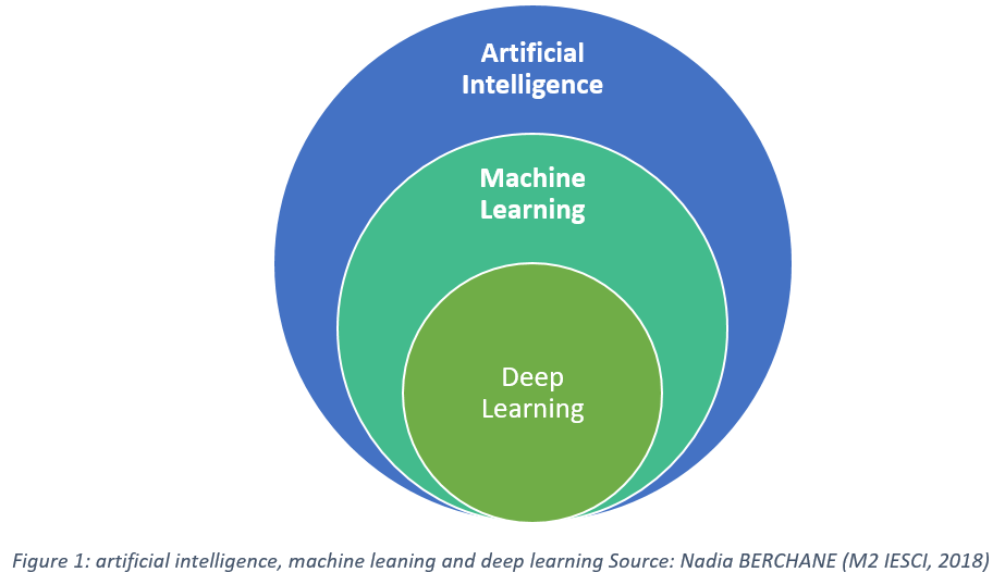
This figure explains the relationship between AI, ML, and Deep Learning. As we can see, AI is the overarching concept, and ML is a big portion of AI, and Deep Learning is finally a subset of ML.
Machine Learning is the practice of using algorithms to analyze data, learn from that data, and then make a determination or prediction about new data. This notebook will introduce Deep Learning, which is a subset of machine learning that attempts to build algorithms called neural networks, which model the structure of the human brain.
You may be wondering what the difference between ML and standard programming. For example, if we are building an AI assistant, such as Siri, why can't we just use if-statements and other logic to answer questions.
If we think about it a bit more, we realize that there are so many different questions you can ask Siri, and it would be impossible to program an answer to an infinte amount of questions. This means that using traditional programming would not work, and a new approach is needed, which can be Machine Learning
Example: Analyzing the sentament of a popular media outlet and classifying that sentiment as positive or negative
Traditional Programming approach
Machine Learning approach

This figure explains the relationship between AI, ML, and Deep Learning. As we can see, AI is the overarching concept, and ML is a big portion of AI, and Deep Learning is finally a subset of ML.
This lesson will cover the most basic idea about what deep learning is and how it’s used. In later lessons, we’ll be cover more detailed concepts, terms, and tools within the field of deep learning.
Definition:
Supervised Learning occurs when your deep learning model learns and makes inferences from data that has already been labeled. A label is basically an explanation of what the data is. If we have a picture of a dog and we are trying to classify between cats and dogs, the labels for each would be "cats" and "dogs."
Unsupervised Learning occurs when the model learns and makes inferences from unlabeled data. This means we only have data points but no labels for this. This makes learning from this data much more challenging.
Semi-Supervised Learning occurs when the model has data points with labels and data points without labels. This is a mix of supervised and unsupervised learning because we need supervised methods to use the labeled data and unsupervised methods to use the unlabeled data.
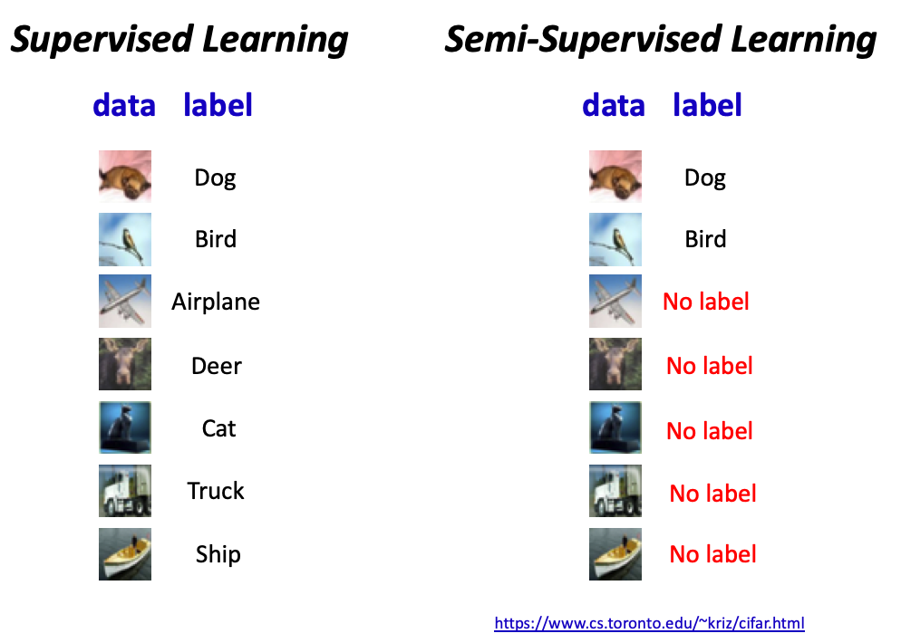
Labeled vs. Unlabeled example
Artificial neural networks are deep learning models that are based on the structure of the brain's neural networks.
Artificial neural networks are computing systems that are inspired by the brain’s neural networks.
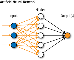
The Sequential model is a linear stack of layers. The following network we coded has 3 layers, the first with 10 nodes, the second with 32, and the last with 2.
from keras.models import Sequential
from keras.layers import Dense, Activation

model = Sequential([
    Dense(32, input_shape=(10,), activation='relu'), # Input Layer
    Dense(2, activation='softmax'), # Output Layer
])
Artificial neural network are typically organized in layers. Different types of layers include (you will learn about these later)
There are different types of layers because each node and each layer does different types of transformations based on its inputs. Some are better for other tasks, such as Convolutional Layers for images or recurreny layers for time series data.
Each node in a layer represents an individual feature for each sample within our dataset. Each input is connected to each node in the hidden layer. The input is then transformed into another output.
Each connection is called a weight. This is just a number 0-1, it is the strength of the connection between the nodes. The input will be multiplied by the input, and a weighted sum of every weight will be calculated, and that is passed to an activation function that will transform the result to a number 0-1. This is a per nueron basis.
That result is then passed on to the next neuron in the next layer, occurs over and over until it gets to the output.
The model learns how to adjust these weights so that it is omptimized and can make the best predictions.
The last layer contains as many nodes as there are classes. For example, if it was predicting if a drawing was a number 0-9, there would be 10 nodes, and if it was if the picture is a cat or dog, it would have two outputs.
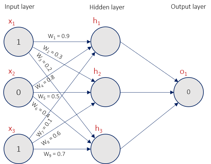
from keras.models import Sequential
from keras.layers import Dense, Activation

model = Sequential([
    Dense(5, input_shape=(3,), activation='relu'),
    Dense(2, activation='softmax'),
])
import numpy as np
from scipy import ndimage
import matplotlib.pyplot as plt
%matplotlib inline

img = np.expand_dims(ndimage.imread('NN.PNG'),0)
plt.imshow(img[0])
<matplotlib.image.AxesImage at 0x7f0b8ba3ac50>
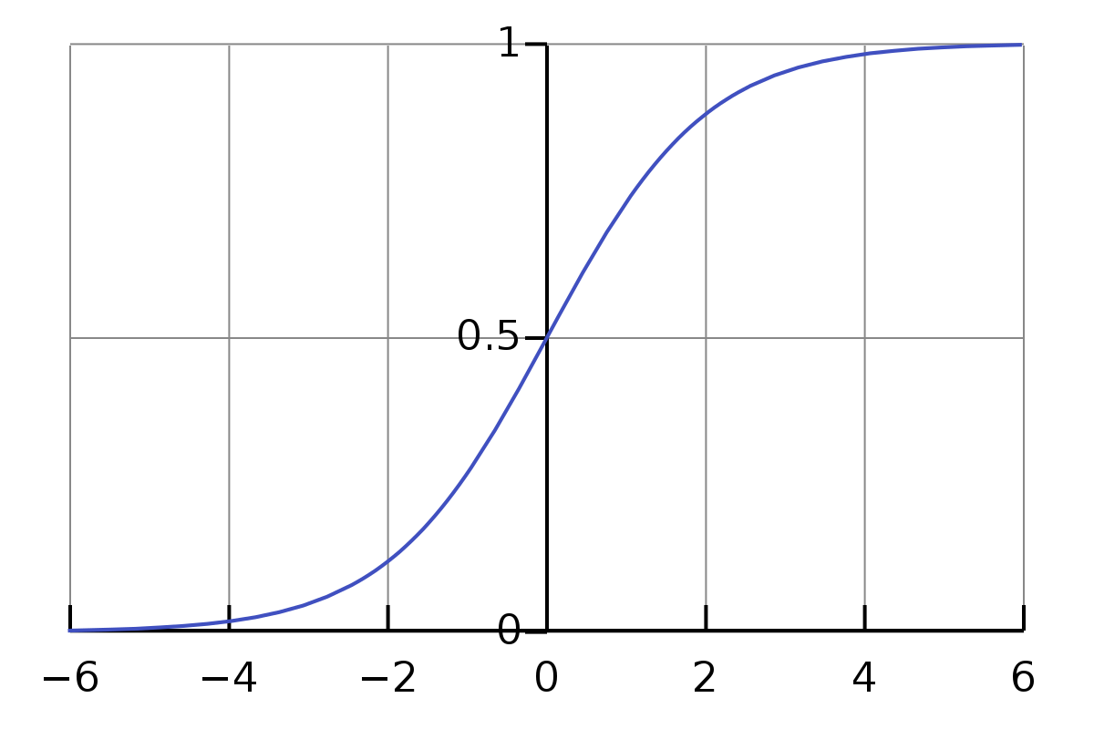
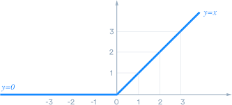
In an artificial neural network, the activation function of a neuron defines the output of that neuron given a set of inputs.
from keras.models import Sequential
from keras.layers import Dense, Activation

model = Sequential([
    Dense(5, input_shape=(3,), activation='relu')
])
model = Sequential()
model.add(Dense(5, input_shape=(3,)))
model.add(Activation('relu'))
Data isn't always going to be given to you in a proper format. You will have to process the data and standarize them, which means make them all the same size, and various other tasks. However, if this is challenging, do not worry, because this isn't technically machine learning or AI. It is rather part of data science, which goes hand in hand with AI/ML. This can be tedious, but you will learn more syntax and strategies as you practice more.
import numpy as np
from random import randint
from sklearn.preprocessing import MinMaxScaler
train_labels =  []
train_samples = []
Example data:
for i in range(50):
    # The 5% of younger individuals who did experience side effects
    random_younger = randint(13,64)
    train_samples.append(random_younger)
    train_labels.append(1)

    # The 5% of older individuals who did not experience side effects
    random_older = randint(65,100)
    train_samples.append(random_older)
    train_labels.append(0)

for i in range(1000):
    # The 95% of younger individuals who did not experience side effects
    random_younger = randint(13,64)
    train_samples.append(random_younger)
    train_labels.append(0)

    # The 95% of older individuals who did experience side effects
    random_older = randint(65,100)
    train_samples.append(random_older)
    train_labels.append(1)
train_labels = np.array(train_labels)
train_samples = np.array(train_samples)
scaler = MinMaxScaler(feature_range=(0,1))
scaled_train_samples = scaler.fit_transform((train_samples).reshape(-1,1))
/home/epoch/anaconda2/envs/fastai34/lib/python3.4/site-packages/sklearn/utils/validation.py:429: DataConversionWarning: Data with input dtype int64 was converted to float64 by MinMaxScaler.
  warnings.warn(msg, _DataConversionWarning)
import numpy as np
from scipy import ndimage
import matplotlib.pyplot as plt
%matplotlib inline

img = np.expand_dims(ndimage.imread('NN.PNG'),0)
plt.imshow(img[0])
<matplotlib.image.AxesImage at 0x7f0b8b576588>
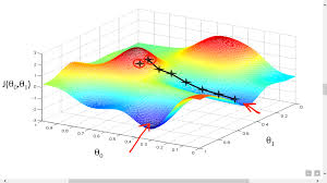
Solving an optimization problem
import keras
from keras import backend as K
from keras.models import Sequential
from keras.layers import Activation
from keras.layers.core import Dense
from keras.optimizers import Adam
from keras.metrics import categorical_crossentropy
model = Sequential([
    Dense(16, input_shape=(1,), activation='relu'),
    Dense(32, activation='relu'),
    Dense(2, activation='sigmoid')
])
model.compile(Adam(lr=.0001), loss='sparse_categorical_crossentropy', metrics=['accuracy'])
model.loss = 'sparse_categorical_crossentropy'
model.loss
'sparse_categorical_crossentropy'
A learning rate is just a way of reducing the gradient so it makes incremental and small adjustments. We are basically explaining by what factor we should change our weights in order to optimize them.
d(loss)/d(weight) * lr(0.001)
To reduce your error, you have to take steps. The learning rate is basically the steps.
d(loss)/ d(weightValue) * lr(0.001) = y Then you replace that current weight with weight - y.
You have to test and tune to find the best learning rate, but the guidlines are to set it between 0.01 and 0.0001. Setting it too high will overshoot and pass the minimum of the loss function. However, with a lower learning rate, it will take a long time to decrease the loss.
model.compile(Adam(lr=0.0001), loss='sparse_categorical_crossentropy', metrics=['accuracy'])
model.optimizer.lr = 0.01
model.optimizer.lr
0.01
model.fit(scaled_train_samples, train_labels, batch_size=10, epochs=20, shuffle=True, verbose=2)
Epoch 1/20
0s - loss: 0.6400 - acc: 0.5576
Epoch 2/20
0s - loss: 0.6061 - acc: 0.6310
Epoch 3/20
0s - loss: 0.5748 - acc: 0.7010
Epoch 4/20
0s - loss: 0.5401 - acc: 0.7633
Epoch 5/20
0s - loss: 0.5050 - acc: 0.7990
Epoch 6/20
0s - loss: 0.4702 - acc: 0.8300
Epoch 7/20
0s - loss: 0.4366 - acc: 0.8495
Epoch 8/20
0s - loss: 0.4066 - acc: 0.8767
Epoch 9/20
0s - loss: 0.3808 - acc: 0.8814
Epoch 10/20
0s - loss: 0.3596 - acc: 0.8962
Epoch 11/20
0s - loss: 0.3420 - acc: 0.9043
Epoch 12/20
0s - loss: 0.3282 - acc: 0.9090
Epoch 13/20
0s - loss: 0.3170 - acc: 0.9129
Epoch 14/20
0s - loss: 0.3081 - acc: 0.9210
Epoch 15/20
0s - loss: 0.3014 - acc: 0.9190
Epoch 16/20
0s - loss: 0.2959 - acc: 0.9205
Epoch 17/20
0s - loss: 0.2916 - acc: 0.9238
Epoch 18/20
0s - loss: 0.2879 - acc: 0.9267
Epoch 19/20
0s - loss: 0.2848 - acc: 0.9252
Epoch 20/20
0s - loss: 0.2824 - acc: 0.9286
<keras.callbacks.History at 0x7f0b82249898>
An overall loss will be collected, based off the difference between the prediction the model gave and the actual label value.
error = output - true = 0.25 - 0 = 0.25
One example is Mean Squared Error(MSE) = square each error for each piece of data, and then average them, and that is the loss. There are lots of different loss functions with different equations and calculations, but they don't really matter right now.

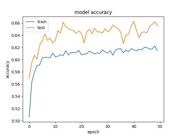
Train, test, and validation sets, all three are part of the entire dataset.
A training set is used for the model to learn from. You give it a piece of data, say an image, and it will predict an output, see the label of that output, and then it will learn how it needs to fix it.
A validation set is used during each pass of the entire data. Once all the data has been given to the model, based on what it has learned, it will make predictions on new data it didn't see for training. This gives a good gague of the accuracy of the model on data it hasn't seen. The weights of the model will not be updated based on the validation set.
The test set is unlabeled, and it is used to determine how your model is doing after it is completely trained.

scaled_train_samples
array([[ 0.27586207],
       [ 0.87356322],
       [ 0.26436782],
       ...,
       [ 0.96551724],
       [ 0.2183908 ],
       [ 0.75862069]])
This is an array of data, they are converted into decimals
train_labels
array([1, 0, 1, ..., 1, 0, 1])
This is a binary classification problem. 1 means a positive label and 0 means a negative label.
model.fit(scaled_train_samples, train_labels, validation_split = 0.20, batch_size=10,
          epochs=20, shuffle=True, verbose=2)
Train on 1680 samples, validate on 420 samples
Epoch 1/20
0s - loss: 0.6994 - acc: 0.4970 - val_loss: 0.6960 - val_acc: 0.5000
Epoch 2/20
0s - loss: 0.6906 - acc: 0.5774 - val_loss: 0.6815 - val_acc: 0.6952
Epoch 3/20
0s - loss: 0.6754 - acc: 0.7179 - val_loss: 0.6613 - val_acc: 0.7857
Epoch 4/20
0s - loss: 0.6548 - acc: 0.7720 - val_loss: 0.6341 - val_acc: 0.8333
Epoch 5/20
0s - loss: 0.6296 - acc: 0.7958 - val_loss: 0.6001 - val_acc: 0.8571
Epoch 6/20
0s - loss: 0.5951 - acc: 0.8161 - val_loss: 0.5516 - val_acc: 0.8714
Epoch 7/20
0s - loss: 0.5545 - acc: 0.8250 - val_loss: 0.5004 - val_acc: 0.8881
Epoch 8/20
0s - loss: 0.5091 - acc: 0.8446 - val_loss: 0.4400 - val_acc: 0.9119
Epoch 9/20
0s - loss: 0.4637 - acc: 0.8726 - val_loss: 0.3886 - val_acc: 0.9310
Epoch 10/20
0s - loss: 0.4283 - acc: 0.8798 - val_loss: 0.3454 - val_acc: 0.9381
Epoch 11/20
0s - loss: 0.3997 - acc: 0.8863 - val_loss: 0.3096 - val_acc: 0.9524
Epoch 12/20
0s - loss: 0.3776 - acc: 0.8917 - val_loss: 0.2805 - val_acc: 0.9524
Epoch 13/20
0s - loss: 0.3602 - acc: 0.8988 - val_loss: 0.2572 - val_acc: 0.9643
Epoch 14/20
0s - loss: 0.3467 - acc: 0.9083 - val_loss: 0.2369 - val_acc: 0.9643
Epoch 15/20
0s - loss: 0.3364 - acc: 0.9113 - val_loss: 0.2214 - val_acc: 0.9643
Epoch 16/20
0s - loss: 0.3288 - acc: 0.9119 - val_loss: 0.2083 - val_acc: 0.9714
Epoch 17/20
0s - loss: 0.3227 - acc: 0.9155 - val_loss: 0.1971 - val_acc: 0.9643
Epoch 18/20
0s - loss: 0.3182 - acc: 0.9137 - val_loss: 0.1889 - val_acc: 0.9786
Epoch 19/20
0s - loss: 0.3144 - acc: 0.9167 - val_loss: 0.1809 - val_acc: 0.9714
Epoch 20/20
0s - loss: 0.3115 - acc: 0.9161 - val_loss: 0.1749 - val_acc: 0.9714
<keras.callbacks.History at 0x7f0b7ec2ee10>
valid_set = [(sample, label), (sample, label), ... , (sample, label)]
model.fit(scaled_train_samples, train_labels, validation_data = valid_set, batch_size=10,
          epochs=20, shuffle=True, verbose=2)
import keras
from keras import backend as K
from keras.models import Sequential
from keras.layers import Activation
from keras.layers.core import Dense
from keras.optimizers import Adam
from keras.metrics import categorical_crossentropy
model = Sequential([
    Dense(16, input_shape=(1,), activation='relu'),
    Dense(32, activation='relu'),
    Dense(2, activation='sigmoid')
])
model.compile(Adam(lr=.0001), loss='sparse_categorical_crossentropy', metrics=['accuracy'])
model.fit(scaled_train_samples, train_labels, batch_size=10, epochs=20, shuffle=True, verbose=2)
Epoch 1/20
0s - loss: 0.6933 - acc: 0.6419
Epoch 2/20
0s - loss: 0.6710 - acc: 0.7857
Epoch 3/20
0s - loss: 0.6397 - acc: 0.8443
Epoch 4/20
0s - loss: 0.6061 - acc: 0.8476
Epoch 5/20
0s - loss: 0.5678 - acc: 0.8505
Epoch 6/20
0s - loss: 0.5228 - acc: 0.8600
Epoch 7/20
0s - loss: 0.4681 - acc: 0.8733
Epoch 8/20
0s - loss: 0.4105 - acc: 0.8962
Epoch 9/20
0s - loss: 0.3670 - acc: 0.9119
Epoch 10/20
0s - loss: 0.3329 - acc: 0.9167
Epoch 11/20
0s - loss: 0.3100 - acc: 0.9243
Epoch 12/20
0s - loss: 0.2925 - acc: 0.9271
Epoch 13/20
0s - loss: 0.2820 - acc: 0.9300
Epoch 14/20
0s - loss: 0.2757 - acc: 0.9338
Epoch 15/20
0s - loss: 0.2712 - acc: 0.9319
Epoch 16/20
0s - loss: 0.2681 - acc: 0.9381
Epoch 17/20
0s - loss: 0.2655 - acc: 0.9376
Epoch 18/20
0s - loss: 0.2634 - acc: 0.9352
Epoch 19/20
0s - loss: 0.2618 - acc: 0.9390
Epoch 20/20
0s - loss: 0.2603 - acc: 0.9352
<keras.callbacks.History at 0x7fa8f1d9fb38>
# Preprocess test data

test_labels =  []
test_samples = []

for i in range(10):
    # The 5% of younger individuals who did experience side effects
    random_younger = randint(13,64)
    test_samples.append(random_younger)
    test_labels.append(1)

    # The 5% of older individuals who did not experience side effects
    random_older = randint(65,100)
    test_samples.append(random_older)
    test_labels.append(0)

for i in range(200):
    # The 95% of younger individuals who did not experience side effects
    random_younger = randint(13,64)
    test_samples.append(random_younger)
    test_labels.append(0)

    # The 95% of older individuals who did experience side effects
    random_older = randint(65,100)
    test_samples.append(random_older)
    test_labels.append(1)

test_labels = np.array(test_labels)
test_samples = np.array(test_samples)

scaler = MinMaxScaler(feature_range=(0,1))
scaled_test_samples = scaler.fit_transform((test_samples).reshape(-1,1))
/home/epoch/anaconda2/envs/fastai34/lib/python3.4/site-packages/sklearn/utils/validation.py:429: DataConversionWarning: Data with input dtype int64 was converted to float64 by MinMaxScaler.
  warnings.warn(msg, _DataConversionWarning)
predictions = model.predict(scaled_test_samples, batch_size=10, verbose=0)
for i in predictions:
    print(i)
[ 0.28293326  0.35764667]
[ 0.26525486  0.37844887]
[ 0.85707456  0.04403995]
[ 0.0979089   0.67903334]
[ 0.87152088  0.04061354]
[ 0.04943148  0.85192239]
[ 0.880009   0.0379883]
[ 0.12007324  0.61951774]
[ 0.64052224  0.10959   ]
[ 0.13958886  0.5766331 ]
[ 0.82027066  0.0517699 ]
[ 0.04943148  0.85192239]
[ 0.87042195  0.04095384]
[ 0.23208363  0.42135212]
[ 0.77739257  0.06212683]
[ 0.23208363  0.42135212]
[ 0.8121165   0.05363343]
[ 0.06808709  0.7811752 ]
[ 0.85707456  0.04403995]
[ 0.0430468   0.87568933]
[ 0.880009   0.0379883]
[ 0.18797709  0.48778817]
[ 0.83300829  0.04906356]
[ 0.07451599  0.7569769 ]
[ 0.32034045  0.31766897]
[ 0.24829839  0.39970824]
[ 0.85979176  0.04345375]
[ 0.09193034  0.69722801]
[ 0.87477005  0.0396088 ]
[ 0.10429112  0.66016704]
[ 0.42364404  0.22938529]
[ 0.21662255  0.44330263]
[ 0.84821194  0.04590416]
[ 0.0430468   0.87568933]
[ 0.82027066  0.0517699 ]
[ 0.06808709  0.7811752 ]
[ 0.87042195  0.04095384]
[ 0.04120404  0.88207549]
[ 0.86930537  0.04130033]
[ 0.20192057  0.46547687]
[ 0.64052224  0.10959   ]
[ 0.04120404  0.88207549]
[ 0.87477005  0.0396088 ]
[ 0.04943148  0.85192239]
[ 0.87152088  0.04061354]
[ 0.26525486  0.37844887]
[ 0.87583733  0.03927922]
[ 0.05176451  0.84311408]
[ 0.84821194  0.04590416]
[ 0.13958886  0.5766331 ]
[ 0.40210381  0.24557945]
[ 0.18797709  0.48778817]
[ 0.67980295  0.09405305]
[ 0.03638967  0.89756322]
[ 0.87152088  0.04061354]
[ 0.04719836  0.86031818]
[ 0.82027066  0.0517699 ]
[ 0.0430468   0.87568933]
[ 0.8768968   0.03895227]
[ 0.13958886  0.5766331 ]
[ 0.36020902  0.28021055]
[ 0.07808454  0.74381268]
[ 0.87794852  0.03862793]
[ 0.21662255  0.44330263]
[ 0.46752542  0.1992964 ]
[ 0.05420133  0.83388394]
[ 0.87152088  0.04061354]
[ 0.13958886  0.5766331 ]
[ 0.7155025   0.08153573]
[ 0.0594027   0.81412745]
[ 0.36020902  0.28021055]
[ 0.16233467  0.53246796]
[ 0.86509645  0.04230364]
[ 0.09193034  0.69722801]
[ 0.87477005  0.0396088 ]
[ 0.24829839  0.39970824]
[ 0.64052224  0.10959   ]
[ 0.06217557  0.80358917]
[ 0.83300829  0.04906356]
[ 0.21662255  0.44330263]
[ 0.40210381  0.24557945]
[ 0.08204049  0.72956663]
[ 0.76366335  0.06596307]
[ 0.05674605  0.82422394]
[ 0.87042195  0.04095384]
[ 0.0430468   0.87568933]
[ 0.86246562  0.04287501]
[ 0.07808454  0.74381268]
[ 0.87152088  0.04061354]
[ 0.04120404  0.88207549]
[ 0.32034045  0.31766897]
[ 0.0430468   0.87568933]
[ 0.83300829  0.04906356]
[ 0.18797709  0.48778817]
[ 0.87583733  0.03927922]
[ 0.0594027   0.81412745]
[ 0.83300829  0.04906356]
[ 0.20192057  0.46547687]
[ 0.62010962  0.11817335]
[ 0.13958886  0.5766331 ]
[ 0.55611736  0.14823376]
[ 0.23208363  0.42135212]
[ 0.87042195  0.04095384]
[ 0.08658814  0.71420431]
[ 0.30130684  0.33736712]
[ 0.05176451  0.84311408]
[ 0.84330875  0.04692649]
[ 0.21662255  0.44330263]
[ 0.87042195  0.04095384]
[ 0.16233467  0.53246796]
[ 0.42364404  0.22938529]
[ 0.03793108  0.89261192]
[ 0.84821194  0.04590416]
[ 0.16233467  0.53246796]
[ 0.84821194  0.04590416]
[ 0.0430468   0.87568933]
[ 0.36020902  0.28021055]
[ 0.21662255  0.44330263]
[ 0.7485773   0.07064888]
[ 0.0594027   0.81412745]
[ 0.59926307  0.12733285]
[ 0.23208363  0.42135212]
[ 0.87477005  0.0396088 ]
[ 0.04120404  0.88207549]
[ 0.48969987  0.18540421]
[ 0.05176451  0.84311408]
[ 0.87477005  0.0396088 ]
[ 0.08204049  0.72956663]
[ 0.82027066  0.0517699 ]
[ 0.0594027   0.81412745]
[ 0.32034045  0.31766897]
[ 0.09193034  0.69722801]
[ 0.80109262  0.05631671]
[ 0.05420133  0.83388394]
[ 0.7155025   0.08153573]
[ 0.12007324  0.61951774]
[ 0.87794852  0.03862793]
[ 0.07808454  0.74381268]
[ 0.87794852  0.03862793]
[ 0.05420133  0.83388394]
[ 0.86930537  0.04130033]
[ 0.0594027   0.81412745]
[ 0.77739257  0.06212683]
[ 0.05674605  0.82422394]
[ 0.85979176  0.04345375]
[ 0.21662255  0.44330263]
[ 0.78949356  0.05915147]
[ 0.03793108  0.89261192]
[ 0.40210381  0.24557945]
[ 0.10429112  0.66016704]
[ 0.48969987  0.18540421]
[ 0.09193034  0.69722801]
[ 0.83827734  0.04797048]
[ 0.04120404  0.88207549]
[ 0.66043848  0.10155829]
[ 0.06217557  0.80358917]
[ 0.78949356  0.05915147]
[ 0.04719836  0.86031818]
[ 0.8736949   0.03994104]
[ 0.12925252  0.59830874]
[ 0.64052224  0.10959   ]
[ 0.0979089   0.67903334]
[ 0.85298848  0.04490304]
[ 0.26525486  0.37844887]
[ 0.40210381  0.24557945]
[ 0.06217557  0.80358917]
[ 0.36020902  0.28021055]
[ 0.03953509  0.88745135]
[ 0.86930537  0.04130033]
[ 0.1117581   0.64022535]
[ 0.82682848  0.05037352]
[ 0.16233467  0.53246796]
[ 0.48969987  0.18540421]
[ 0.06506889  0.7926057 ]
[ 0.82027066  0.0517699 ]
[ 0.05674605  0.82422394]
[ 0.76366335  0.06596307]
[ 0.04719836  0.86031818]
[ 0.85979176  0.04345375]
[ 0.12007324  0.61951774]
[ 0.8768968   0.03895227]
[ 0.07451599  0.7569769 ]
[ 0.55611736  0.14823376]
[ 0.04943148  0.85192239]
[ 0.55611736  0.14823376]
[ 0.0430468   0.87568933]
[ 0.33999148  0.29860252]
[ 0.03793108  0.89261192]
[ 0.86509645  0.04230364]
[ 0.23208363  0.42135212]
[ 0.4454785   0.21395613]
[ 0.08204049  0.72956663]
[ 0.82682848  0.05037352]
[ 0.24829839  0.39970824]
[ 0.86246562  0.04287501]
[ 0.21662255  0.44330263]
[ 0.87898576  0.03830663]
[ 0.0979089   0.67903334]
[ 0.82682848  0.05037352]
[ 0.08204049  0.72956663]
[ 0.880009   0.0379883]
[ 0.07808454  0.74381268]
[ 0.33999148  0.29860252]
[ 0.03793108  0.89261192]
[ 0.82027066  0.0517699 ]
[ 0.0594027   0.81412745]
[ 0.87042195  0.04095384]
[ 0.13958886  0.5766331 ]
[ 0.87261182  0.04027594]
[ 0.05674605  0.82422394]
[ 0.78949356  0.05915147]
[ 0.09193034  0.69722801]
[ 0.38093486  0.26252744]
[ 0.12007324  0.61951774]
[ 0.87583733  0.03927922]
[ 0.0979089   0.67903334]
[ 0.8768968   0.03895227]
[ 0.04719836  0.86031818]
[ 0.8676846   0.04173953]
[ 0.05420133  0.83388394]
[ 0.55611736  0.14823376]
[ 0.06217557  0.80358917]
[ 0.42364404  0.22938529]
[ 0.21662255  0.44330263]
[ 0.76366335  0.06596307]
[ 0.05674605  0.82422394]
[ 0.880009   0.0379883]
[ 0.24829839  0.39970824]
[ 0.83827734  0.04797048]
[ 0.12925252  0.59830874]
[ 0.36020902  0.28021055]
[ 0.08204049  0.72956663]
[ 0.86509645  0.04230364]
[ 0.04506137  0.86831146]
[ 0.87261182  0.04027594]
[ 0.04506137  0.86831146]
[ 0.86509645  0.04230364]
[ 0.17478551  0.51014841]
[ 0.7155025   0.08153573]
[ 0.0430468   0.87568933]
[ 0.33999148  0.29860252]
[ 0.07808454  0.74381268]
[ 0.8736949   0.03994104]
[ 0.0594027   0.81412745]
[ 0.4454785   0.21395613]
[ 0.12925252  0.59830874]
[ 0.85707456  0.04403995]
[ 0.0430468   0.87568933]
[ 0.67980295  0.09405305]
[ 0.18797709  0.48778817]
[ 0.62010962  0.11817335]
[ 0.03953509  0.88745135]
[ 0.62010962  0.11817335]
[ 0.05420133  0.83388394]
[ 0.80109262  0.05631671]
[ 0.09193034  0.69722801]
[ 0.85298848  0.04490304]
[ 0.20192057  0.46547687]
[ 0.83300829  0.04906356]
[ 0.10429112  0.66016704]
[ 0.62010962  0.11817335]
[ 0.06506889  0.7926057 ]
[ 0.55611736  0.14823376]
[ 0.04506137  0.86831146]
[ 0.85707456  0.04403995]
[ 0.04506137  0.86831146]
[ 0.55611736  0.14823376]
[ 0.06808709  0.7811752 ]
[ 0.8768968   0.03895227]
[ 0.08204049  0.72956663]
[ 0.64052224  0.10959   ]
[ 0.07451599  0.7569769 ]
[ 0.8736949   0.03994104]
[ 0.0430468   0.87568933]
[ 0.76366335  0.06596307]
[ 0.06808709  0.7811752 ]
[ 0.69801664  0.08753506]
[ 0.05674605  0.82422394]
[ 0.4454785   0.21395613]
[ 0.04719836  0.86031818]
[ 0.87152088  0.04061354]
[ 0.03638967  0.89756322]
[ 0.85979176  0.04345375]
[ 0.15060882  0.55465847]
[ 0.83827734  0.04797048]
[ 0.18797709  0.48778817]
[ 0.87477005  0.0396088 ]
[ 0.10429112  0.66016704]
[ 0.32034045  0.31766897]
[ 0.03953509  0.88745135]
[ 0.8736949   0.03994104]
[ 0.20192057  0.46547687]
[ 0.732364    0.07591337]
[ 0.03793108  0.89261192]
[ 0.880009   0.0379883]
[ 0.1117581   0.64022535]
[ 0.85707456  0.04403995]
[ 0.04943148  0.85192239]
[ 0.87794852  0.03862793]
[ 0.0430468   0.87568933]
[ 0.732364    0.07591337]
[ 0.05420133  0.83388394]
[ 0.83827734  0.04797048]
[ 0.16233467  0.53246796]
[ 0.880009   0.0379883]
[ 0.07451599  0.7569769 ]
[ 0.732364    0.07591337]
[ 0.20192057  0.46547687]
[ 0.87152088  0.04061354]
[ 0.03638967  0.89756322]
[ 0.8768968   0.03895227]
[ 0.07808454  0.74381268]
[ 0.87152088  0.04061354]
[ 0.03953509  0.88745135]
[ 0.83827734  0.04797048]
[ 0.0979089   0.67903334]
[ 0.53408301  0.15988748]
[ 0.03793108  0.89261192]
[ 0.77739257  0.06212683]
[ 0.24829839  0.39970824]
[ 0.48969987  0.18540421]
[ 0.04120404  0.88207549]
[ 0.85979176  0.04345375]
[ 0.0430468   0.87568933]
[ 0.7485773   0.07064888]
[ 0.23208363  0.42135212]
[ 0.87583733  0.03927922]
[ 0.06808709  0.7811752 ]
[ 0.84330875  0.04692649]
[ 0.12925252  0.59830874]
[ 0.28293326  0.35764667]
[ 0.04943148  0.85192239]
[ 0.86246562  0.04287501]
[ 0.03793108  0.89261192]
[ 0.46752542  0.1992964 ]
[ 0.0430468   0.87568933]
[ 0.38093486  0.26252744]
[ 0.03953509  0.88745135]
[ 0.87477005  0.0396088 ]
[ 0.23208363  0.42135212]
[ 0.87261182  0.04027594]
[ 0.0594027   0.81412745]
[ 0.82027066  0.0517699 ]
[ 0.12925252  0.59830874]
[ 0.7155025   0.08153573]
[ 0.03638967  0.89756322]
[ 0.86930537  0.04130033]
[ 0.12007324  0.61951774]
[ 0.53408301  0.15988748]
[ 0.21662255  0.44330263]
[ 0.7155025   0.08153573]
[ 0.07808454  0.74381268]
[ 0.67980295  0.09405305]
[ 0.05674605  0.82422394]
[ 0.84821194  0.04590416]
[ 0.0979089   0.67903334]
[ 0.84821194  0.04590416]
[ 0.05176451  0.84311408]
[ 0.87042195  0.04095384]
[ 0.20192057  0.46547687]
[ 0.67980295  0.09405305]
[ 0.18797709  0.48778817]
[ 0.85298848  0.04490304]
[ 0.0430468   0.87568933]
[ 0.77739257  0.06212683]
[ 0.0594027   0.81412745]
[ 0.36020902  0.28021055]
[ 0.24829839  0.39970824]
[ 0.84330875  0.04692649]
[ 0.26525486  0.37844887]
[ 0.40210381  0.24557945]
[ 0.06506889  0.7926057 ]
[ 0.86509645  0.04230364]
[ 0.0594027   0.81412745]
[ 0.30130684  0.33736712]
[ 0.23208363  0.42135212]
[ 0.36020902  0.28021055]
[ 0.04506137  0.86831146]
[ 0.82027066  0.0517699 ]
[ 0.06808709  0.7811752 ]
[ 0.48969987  0.18540421]
[ 0.05420133  0.83388394]
[ 0.4454785   0.21395613]
[ 0.08204049  0.72956663]
[ 0.32034045  0.31766897]
[ 0.0430468   0.87568933]
[ 0.880009   0.0379883]
[ 0.23208363  0.42135212]
[ 0.8121165   0.05363343]
[ 0.08658814  0.71420431]
[ 0.51191491  0.17227209]
[ 0.17478551  0.51014841]
[ 0.8121165   0.05363343]
[ 0.04120404  0.88207549]
[ 0.880009   0.0379883]
[ 0.08204049  0.72956663]
[ 0.87898576  0.03830663]
[ 0.03793108  0.89261192]
[ 0.87042195  0.04095384]
[ 0.06217557  0.80358917]
[ 0.82682848  0.05037352]
[ 0.12007324  0.61951774]
[ 0.77739257  0.06212683]
[ 0.04719836  0.86031818]
[ 0.84330875  0.04692649]
[ 0.06506889  0.7926057 ]
[ 0.87898576  0.03830663]
[ 0.07808454  0.74381268]
[ 0.8736949   0.03994104]
[ 0.07123458  0.76929814]
[ 0.33999148  0.29860252]
[ 0.0430468   0.87568933]
[ 0.85707456  0.04403995]
[ 0.07808454  0.74381268]
[ 0.83827734  0.04797048]
[ 0.04506137  0.86831146]
[ 0.85298848  0.04490304]
[ 0.07123458  0.76929814]
[ 0.42364404  0.22938529]
[ 0.17478551  0.51014841]
model.fit(scaled_train_samples, train_labels, validation_data = valid_set, batch_size=10,
          epochs=20, shuffle=True, verbose=2)
import keras
from keras import backend as K
from keras.models import Sequential
from keras.layers import Activation
from keras.layers.core import Dense
from keras.optimizers import Adam
model = Sequential([
    Dense(16, input_shape=(2,), activation='relu'),
    Dense(32, activation='relu'),
    Dense(2, activation='sigmoid')
])
model.compile(Adam(lr=0.0001), loss='sparse_categorical_crossentropy', metrics=['accuracy'])
# weight, height
train_samples = [[150, 67], [130, 60], [200, 65], [125, 52], [230, 72], [181, 70]]
# 0: male
# 1: female
train_labels = [1, 1, 0, 1, 0, 0]
model.fit(x=train_samples, y=train_labels, batch_size=3, epochs=10, shuffle=True, verbose=2)